Shapefile to GeoJSON Converter: Complete Guide for Web Mapping

You downloaded geographic data from your city’s open data portal. It’s a .zip file containing roads.shp, roads.dbf, roads.shx, and three other files you don’t recognize. You want to display it on your website with Leaflet.js.

But Leaflet doesn’t read shapefiles.

Or maybe you’re building a real estate platform. Your county provides property boundary data—10,000 parcels in ESRI shapefile format. You need to overlay them on an interactive map where users can click properties to see details.

Your JavaScript mapping library expects GeoJSON, not binary shapefile components.

Or perhaps you’re a data journalist preparing an interactive story about election results by district. You have the geographic boundaries from the election commission as shapefiles. Your D3.js visualization needs GeoJSON.

Converting shapefiles manually in GIS software for every dataset is killing your productivity.

Here’s the reality: Shapefiles are the industry standard for desktop GIS, but they’re completely incompatible with modern web mapping. Created by ESRI in the early 1990s, shapefiles require 3-7 separate files, use binary encoding, and need specialized parsers. Meanwhile, every web mapping library—Leaflet, Mapbox GL JS, OpenLayers, Google Maps API—expects GeoJSON: a single, readable JSON file.

The gap between these formats frustrates developers daily. You can’t just rename .shp to .geojson. You need proper conversion that transforms coordinates, preserves attributes, handles projections, and validates geometry.

This guide shows you exactly how to bridge that gap. You’ll learn why shapefiles and GeoJSON exist, how to convert between them using online tools or command-line utilities, integrate converted data into Leaflet and Mapbox, troubleshoot common conversion errors, and optimize GeoJSON files for production web maps.

By the end, you’ll convert any shapefile to web-ready GeoJSON in under 30 seconds—and understand what’s happening under the hood.

Quick Answer: Converting Shapefiles to GeoJSON

Don’t have time for 7,000 words? Here’s what you need to know:

What you need: Minimum 3 files (.shp, .shx, .dbf) plus optional .prj for accurate coordinates
Best online tool: Use our Shapefile Converter for instant conversion up to 50MB
Command-line option: ogr2ogr -f GeoJSON output.geojson input.shp (requires GDAL)
Desktop software: QGIS (free) exports shapefiles to GeoJSON in 3 clicks
Key difference: Shapefiles = binary, multi-file, desktop GIS | GeoJSON = JSON, single file, web mapping
Common mistake: Missing .prj file causes coordinates to appear in wrong location
File size: GeoJSON is 40-60% larger than shapefile, but compresses well with gzip
Web integration: L.geoJSON(data).addTo(map) works immediately in Leaflet

Ready to master shapefile conversion? Let’s dive in.

What Are Shapefiles and Why Can’t Browsers Read Them?

Understanding ESRI Shapefiles

A shapefile is a geospatial vector data format developed by ESRI (Environmental Systems Research Institute) in the early 1990s. Despite being 30+ years old, it remains the most widely-used format for exchanging GIS data.

Here’s the catch: “Shapefile” is misleading. It’s not one file—it’s a collection of multiple files that work together.

The Multi-File Nightmare

When you download a shapefile, you actually get at least 3 files (often 5-7):

Required Files (Can’t work without all 3):

.shp - Shape Format File
- Contains the actual geometry (points, lines, polygons)
- Stores coordinate pairs for every vertex
- Binary format, not human-readable
.shx - Shape Index File
- Positional index linking geometry to attributes
- Enables fast spatial queries
- Critical for performance
.dbf - dBase Attribute Table
- Stores feature attributes in columnar format
- Example: street names, population counts, land use codes
- Based on 1980s dBase database format
- Major limitation: Column names limited to 10 characters

Optional But Important:
4. .prj - Projection File

Defines coordinate reference system (CRS)
Critical: Missing this file causes conversion errors
Example: WGS84, NAD83 State Plane, UTM zones

.cpg - Code Page File
- Specifies character encoding (UTF-8, Windows-1252, etc.)
- Prevents garbled text in international datasets
.sbn / .sbx - Spatial Index (created by ArcGIS)

Shapefile Upload Interface

Why Browsers Can’t Use Shapefiles

Binary Format Problem:
Shapefiles use binary encoding designed for desktop software, not browsers. JavaScript can’t natively parse .shp files without specialized libraries.

Multi-File Dependency:
Web applications work with single-file formats (JSON, XML, CSV). Managing 3-7 interdependent files breaks web workflows.

No Native Support:
Unlike JSON (which every browser parses natively), shapefiles require external parsers that add ~100KB to your bundle.

Desktop-First Design:
Shapefiles were designed for desktop GIS workflows: ArcGIS, QGIS, MapInfo. The web didn’t exist when ESRI created the format in 1991.

Real-World Impact

Example scenario: You download a 10MB shapefile of city boundaries from data.gov. Here’s what you face:

city-boundaries.zip contains:
  ├── boundaries.shp    (6.2 MB)
  ├── boundaries.shx    (0.8 MB)
  ├── boundaries.dbf    (2.4 MB)
  ├── boundaries.prj    (171 bytes)
  └── boundaries.cpg    (5 bytes)

Your Leaflet.js code:

// This doesn't work!
fetch('boundaries.shp')
  .then(response => response.json())  // ❌ Fails - binary format
  .then(data => L.geoJSON(data).addTo(map));

You need conversion first.

What is GeoJSON and Why Do Web Maps Love It?

Understanding GeoJSON

GeoJSON is an open standard format (RFC 7946) for encoding geographic data structures using JSON (JavaScript Object Notation). It was specifically designed for web applications.

Published: October 2016 by the Internet Engineering Task Force (IETF)
File extension: .geojson or .json
MIME type: application/geo+json

Why GeoJSON Wins for Web Mapping

1. Native Browser Support

// Works immediately - no special libraries
fetch('data.geojson')
  .then(response => response.json())  // ✅ Native JSON parsing
  .then(data => L.geoJSON(data).addTo(map));

2. Single File Format

city-boundaries.geojson  (4.1 MB)

One file contains everything: geometry + attributes + metadata.

3. Human-Readable
Open in any text editor to inspect, debug, or modify:

{
  "type": "FeatureCollection",
  "features": [
    {
      "type": "Feature",
      "geometry": {
        "type": "Polygon",
        "coordinates": [[[-122.4194, 37.7749], ...]]
      },
      "properties": {
        "name": "San Francisco",
        "population": 873965,
        "area_sqkm": 600.6
      }
    }
  ]
}

4. Universal Library Support

Leaflet.js: L.geoJSON(data)
Mapbox GL JS: map.addSource('data', {type: 'geojson', data: data})
OpenLayers: new VectorSource({format: new GeoJSON()})
D3.js: d3.geoPath().projection(projection)(geojson)
Google Maps: map.data.addGeoJson(data)

5. API-Friendly
Perfect for RESTful APIs:

GET /api/properties?city=SF
Response: application/geo+json

GeoJSON Structure Breakdown

Basic FeatureCollection:

{
  "type": "FeatureCollection",
  "features": [
    {
      "type": "Feature",
      "id": 1,
      "geometry": {
        "type": "Point",
        "coordinates": [-122.4194, 37.7749]
      },
      "properties": {
        "city": "San Francisco",
        "state": "California",
        "population": 873965
      }
    }
  ]
}

Supported Geometry Types:

Point - Single coordinate
LineString - Array of coordinates (roads, routes)
Polygon - Array of linear rings (boundaries, buildings)
MultiPoint - Multiple unconnected points
MultiLineString - Multiple separate lines
MultiPolygon - Multiple separate polygons (island chains)
GeometryCollection - Mixed geometry types

Coordinate Order (CRITICAL):

[longitude, latitude, altitude]

Not [latitude, longitude] like many assume. This trips up developers constantly.

The Mandatory Coordinate System

RFC 7946 specifies that GeoJSON must use WGS84 (EPSG:4326):

Longitude: -180° to +180°
Latitude: -90° to +90°
Datum: WGS84 (same as GPS)

This is non-negotiable. If your shapefile uses a different coordinate system (State Plane, UTM, Web Mercator), conversion must transform it to WGS84.

Shapefile vs GeoJSON: Technical Comparison

Feature	Shapefile	GeoJSON	Winner
File Structure	Multi-file (3-7 files)	Single JSON file	GeoJSON
Browser Compatibility	None (binary)	Native JSON.parse()	GeoJSON
Human Readable	No (hex viewers only)	Yes (text editor)	GeoJSON
File Size (raw)	Compact binary	40-60% larger	Shapefile
File Size (gzipped)	~Same	~Same	Tie
Desktop GIS Support	Universal	QGIS, ArcGIS Pro 2.2+	Shapefile
Web Mapping	Requires conversion	Direct use	GeoJSON
Column Name Length	10 characters max	Unlimited	GeoJSON
Nested Properties	No (flat table)	Yes (full JSON)	GeoJSON
Coordinate Systems	Any CRS	WGS84 only	Shapefile
Version Control (Git)	Binary diffs useless	Line-by-line diffs	GeoJSON
Data Types	Limited (String, Number, Date)	Full JSON types	GeoJSON
Max File Size	2GB per component	No practical limit	GeoJSON

When to Use Each Format

Use Shapefiles for:

Desktop GIS workflows (ArcGIS, QGIS, AutoCAD)
Data archival (smaller file size)
Sharing with government agencies (required format)
Complex coordinate systems (State Plane, UTM)
High-precision surveying data

Use GeoJSON for:

Web mapping (Leaflet, Mapbox, Google Maps)
API responses
Mobile applications (React Native)
Data visualization (D3.js, Observable)
Version control systems (Git)
NoSQL databases (MongoDB GeoJSON support)

Best Practice: Keep shapefiles as your “source of truth” for data storage and analysis. Convert to GeoJSON only when deploying to web applications. This hybrid approach gives you the best of both worlds.

How to Convert Shapefile to GeoJSON (4 Methods)

Method 1: Online Converter (Easiest)

Best for: Quick conversions, non-technical users, files under 50MB

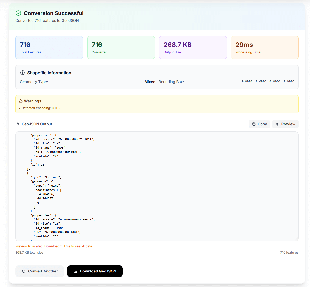
Our Shapefile to GeoJSON Converter handles conversion in your browser:

Step-by-step:

Upload Required Files
- Drag and drop or click to select:
  - filename.shp (geometry)
  - filename.shx (index)
  - filename.dbf (attributes)
- Highly recommended: Include filename.prj (projection)
Configure Options
- Coordinate Precision: 6 decimals (default) = ~10cm accuracy
- Pretty Print: Enable for readable JSON, disable for production
- Validate Geometry: Check for topology errors before deployment
- Include CRS Info: Add coordinate system metadata
Convert
- Processing time: 1-3 seconds for most files
- Preview map shows your data overlaid on basemap
- Verify features render in correct location
Download
- Get RFC 7946-compliant GeoJSON
- Use immediately in web mapping libraries

Conversion Results

Advantages:

No software installation
Works on any device with browser
Live map preview with Leaflet
Automatic projection transformation
Geometry validation included

Limitations:

File size limit (50MB)
Requires internet connection
Data temporarily uploaded to server (deleted after conversion)

Method 2: QGIS (Best for Desktop Users)

Best for: Large files, batch processing, advanced editing

QGIS is free, open-source desktop GIS software available for Windows, Mac, and Linux.

Installation:

# Ubuntu/Debian
sudo apt install qgis

# macOS (Homebrew)
brew install qgis

# Windows
# Download installer from https://qgis.org/download/

Conversion Steps:

Open Shapefile
- Layer → Add Layer → Add Vector Layer
- Browse to .shp file (other components auto-detected)
- Data loads on map canvas
Verify Data
- Check features render correctly
- Open attribute table to verify properties
- Confirm coordinate system in layer properties
Export to GeoJSON
- Right-click layer → Export → Save Features As
- Format: GeoJSON
- CRS: EPSG:4326 - WGS 84
- Coordinate precision: 6 decimals
- Click OK

Advanced Options in Export Dialog:

Layer Options:
- COORDINATE_PRECISION: 6
- RFC7946: YES (strict compliance)
- WRITE_BBOX: YES (include bounding box)

Select Fields to Export:
☑ name
☑ population
☑ area
☐ internal_id (uncheck to exclude)

Batch Conversion Script (Processing Toolbox):

# QGIS Python Console
from processing import run

run("native:reprojectlayer", {
    'INPUT': '/path/to/shapefile.shp',
    'TARGET_CRS': 'EPSG:4326',
    'OUTPUT': '/path/to/output.geojson'
})

Method 3: Command-Line (ogr2ogr)

Best for: Automation, scripting, very large files, production pipelines

ogr2ogr is part of GDAL (Geospatial Data Abstraction Library), the industry-standard tool for geospatial data conversion.

Installation:

# Ubuntu/Debian
sudo apt-get install gdal-bin

# macOS (Homebrew)
brew install gdal

# Windows
# Download from https://gdal.org/download.html
# or use OSGeo4W installer

Verify Installation:

ogr2ogr --version
# Output: GDAL 3.8.3, released 2024/01/04

Basic Conversion:

ogr2ogr -f GeoJSON output.geojson input.shp

Production-Ready Conversion:

ogr2ogr \
  -f GeoJSON \
  -t_srs EPSG:4326 \
  -lco COORDINATE_PRECISION=6 \
  -lco RFC7946=YES \
  -lco WRITE_BBOX=YES \
  output.geojson \
  input.shp

Options Explained:

-f GeoJSON - Output format
-t_srs EPSG:4326 - Transform to WGS84
-lco COORDINATE_PRECISION=6 - 6 decimal places (~10cm accuracy)
-lco RFC7946=YES - Strict RFC 7946 compliance
-lco WRITE_BBOX=YES - Include bounding box in output

Advanced Use Cases:

1. Filter by Attributes:

# Export only cities with population > 100,000
ogr2ogr \
  -f GeoJSON \
  -where "population > 100000" \
  large_cities.geojson \
  cities.shp

2. Select Specific Columns:

# Include only name and population (reduce file size)
ogr2ogr \
  -f GeoJSON \
  -select "name,population,area" \
  filtered.geojson \
  input.shp

3. Simplify Geometry:

# Reduce vertex count for faster rendering
# Tolerance 0.0001 degrees (~11 meters)
ogr2ogr \
  -f GeoJSON \
  -simplify 0.0001 \
  simplified.geojson \
  detailed.shp

4. Reproject from Specific CRS:

# If .prj missing, manually specify source CRS
ogr2ogr \
  -s_srs EPSG:2227 \  # NAD83 California State Plane Zone 3
  -t_srs EPSG:4326 \  # WGS84
  output.geojson \
  input.shp

5. Batch Convert Directory:

#!/bin/bash
# Convert all shapefiles in current directory
for file in *.shp; do
  output="${file%.shp}.geojson"
  ogr2ogr -f GeoJSON -t_srs EPSG:4326 "$output" "$file"
  echo "Converted $file → $output"
done

6. Check Shapefile Info Before Converting:

# View metadata, CRS, feature count, extent
ogrinfo -al -so input.shp

# Output includes:
# - Geometry type
# - Feature count
# - CRS (EPSG code)
# - Bounding box
# - Attribute field names and types

Method 4: Programming Libraries

Best for: Data pipelines, automated workflows, custom processing

Python (GeoPandas)

import geopandas as gpd

# Read shapefile
gdf = gpd.read_file('input.shp')

# Convert to WGS84 if needed
if gdf.crs != 'EPSG:4326':
    gdf = gdf.to_crs('EPSG:4326')

# Export to GeoJSON
gdf.to_file('output.geojson', driver='GeoJSON')

With coordinate precision control:

import json
import geopandas as gpd

gdf = gpd.read_file('input.shp')
gdf = gdf.to_crs('EPSG:4326')

# Convert to GeoJSON string
geojson_str = gdf.to_json()
geojson = json.loads(geojson_str)

# Round coordinates to 6 decimals
def round_coords(coords, precision=6):
    if isinstance(coords[0], list):
        return [round_coords(c, precision) for c in coords]
    return [round(c, precision) for c in coords]

for feature in geojson['features']:
    geom = feature['geometry']
    if geom and 'coordinates' in geom:
        geom['coordinates'] = round_coords(geom['coordinates'], 6)

# Save with indentation for readability
with open('output.geojson', 'w') as f:
    json.dump(geojson, f, indent=2)

Filter and convert:

import geopandas as gpd

# Read and filter
gdf = gpd.read_file('parcels.shp')
valuable = gdf[gdf['assessed_value'] > 1000000]

# Export filtered data
valuable.to_file('high_value_parcels.geojson', driver='GeoJSON')

Node.js

const shapefile = require('shapefile');
const fs = require('fs');

async function convertShapefile(shpPath, geojsonPath) {
  const features = [];

  // Open shapefile
  const source = await shapefile.open(shpPath);

  // Read all features
  let result = await source.read();
  while (!result.done) {
    features.push(result.value);
    result = await source.read();
  }

  // Create FeatureCollection
  const geojson = {
    type: 'FeatureCollection',
    features: features
  };

  // Write to file
  fs.writeFileSync(geojsonPath, JSON.stringify(geojson, null, 2));
  console.log(`Converted ${features.length} features to ${geojsonPath}`);
}

// Usage
convertShapefile('input.shp', 'output.geojson');

Understanding Coordinate Systems and Projection

Why Coordinate Systems Matter

The Problem: Earth is a 3D sphere (technically an oblate spheroid). Maps are 2D. Flattening a sphere onto a plane requires mathematical projection, which introduces distortion.

Different projections optimize for different properties:

Preserve area (equal-area projections)
Preserve shape (conformal projections)
Preserve distance (equidistant projections)
Preserve direction (azimuthal projections)

Real-world impact: If your shapefile uses California State Plane coordinates and you convert without specifying projection, features will render ~200 meters off their true location.

Common Coordinate Reference Systems

WGS84 (EPSG:4326) - Web Standard

Full name: World Geodetic System 1984
Type: Geographic (latitude/longitude)
Units: Degrees
Range: Longitude -180° to 180°, Latitude -90° to 90°
Used by: GPS, Google Maps, all web mapping
Required for: GeoJSON (RFC 7946 mandate)

Example coordinates: [-122.4194, 37.7749]
                     [longitude, latitude]

Web Mercator (EPSG:3857)

Full name: WGS 84 / Pseudo-Mercator
Type: Projected (Cartesian)
Units: Meters
Used by: Google Maps tiles, OpenStreetMap, Bing
Distortion: Extreme at high latitudes (Greenland appears huge)
Note: Cannot be used in GeoJSON (must convert to EPSG:4326)

NAD83 State Plane (US Regional)

Type: Projected (multiple zones)
Units: Feet or meters (varies by zone)
Accuracy: Optimized within state boundaries
Example: California Zone 3 (EPSG:2227)
Common in: US government datasets, county GIS data

UTM (Universal Transverse Mercator)

Type: Projected (60 zones)
Units: Meters
Coverage: 6° wide zones covering globe
Accuracy: High within zone (<0.04% distortion)
Example: UTM Zone 10N (EPSG:32610) covers California

Detecting Coordinate System

Method 1: Check .prj File

# Open .prj file in text editor
cat boundaries.prj

# Output (WGS84 example):
GEOGCS["GCS_WGS_1984",
  DATUM["D_WGS_1984",
    SPHEROID["WGS_1984",6378137,298.257223563]],
  PRIMEM["Greenwich",0],
  UNIT["Degree",0.017453292519943295]]

Method 2: Use ogrinfo

ogrinfo -al -so input.shp | grep -A 5 "Layer SRS WKT"

# Output shows full WKT string and EPSG code

Method 3: QGIS

Load shapefile
Layer Properties → Information → CRS
Shows readable name and EPSG code

Projection Transformation During Conversion

Automatic Transformation (with .prj):

Our converter (and ogr2ogr) automatically:

Reads source CRS from .prj file
Applies mathematical transformation to WGS84
Outputs GeoJSON in EPSG:4326

Manual Transformation (missing .prj):

# Specify source CRS manually
ogr2ogr \
  -s_srs EPSG:2227 \  # Source: California State Plane Zone 3
  -t_srs EPSG:4326 \  # Target: WGS84
  output.geojson \
  input.shp

Verify Transformation:
After conversion, load GeoJSON in geojson.io and verify features render over correct geographic location.

Integrating GeoJSON with Web Mapping Libraries

Leaflet.js (Most Popular)

Leaflet is the leading open-source JavaScript library for mobile-friendly interactive maps. It’s lightweight (39KB gzipped) and easy to learn.

Basic Integration:

<!DOCTYPE html>
<html>
<head>
  <link rel="stylesheet" href="https://unpkg.com/leaflet@1.9.4/dist/leaflet.css" />
  <script src="https://unpkg.com/leaflet@1.9.4/dist/leaflet.js"></script>
  <style>
    #map { height: 600px; }
  </style>
</head>
<body>
  <div id="map"></div>

  <script>
    // Initialize map
    const map = L.map('map').setView([37.7749, -122.4194], 10);

    // Add basemap tiles
    L.tileLayer('https://{s}.tile.openstreetmap.org/{z}/{x}/{y}.png', {
      attribution: '© OpenStreetMap contributors',
      maxZoom: 19
    }).addTo(map);

    // Load and display GeoJSON
    fetch('neighborhoods.geojson')
      .then(response => response.json())
      .then(data => {
        L.geoJSON(data).addTo(map);
      });
  </script>
</body>
</html>

With Custom Styling:

fetch('neighborhoods.geojson')
  .then(response => response.json())
  .then(data => {
    L.geoJSON(data, {
      style: function(feature) {
        return {
          fillColor: getColor(feature.properties.density),
          weight: 2,
          opacity: 1,
          color: 'white',
          fillOpacity: 0.7
        };
      },
      onEachFeature: function(feature, layer) {
        // Add popup with properties
        const props = feature.properties;
        layer.bindPopup(`
          <h3>${props.name}</h3>
          <p>Population: ${props.population.toLocaleString()}</p>
          <p>Density: ${props.density} per sq km</p>
        `);
      }
    }).addTo(map);
  });

// Color function for choropleth map
function getColor(density) {
  return density > 1000 ? '#800026' :
         density > 500  ? '#BD0026' :
         density > 200  ? '#E31A1C' :
         density > 100  ? '#FC4E2A' :
         density > 50   ? '#FD8D3C' :
         density > 20   ? '#FEB24C' :
         density > 10   ? '#FED976' :
                          '#FFEDA0';
}

Point Markers with Custom Icons:

L.geoJSON(data, {
  pointToLayer: function(feature, latlng) {
    // Custom marker icon
    const icon = L.icon({
      iconUrl: 'marker-icon.png',
      iconSize: [25, 41],
      iconAnchor: [12, 41],
      popupAnchor: [1, -34]
    });
    return L.marker(latlng, {icon: icon});
  },
  onEachFeature: function(feature, layer) {
    layer.bindPopup(`<b>${feature.properties.name}</b>`);
  }
}).addTo(map);

Mapbox GL JS

Mapbox GL JS is a powerful WebGL-powered library for vector maps with smooth zoom and rotation.

mapboxgl.accessToken = 'YOUR_MAPBOX_TOKEN';

const map = new mapboxgl.Map({
  container: 'map',
  style: 'mapbox://styles/mapbox/light-v10',
  center: [-122.4194, 37.7749],
  zoom: 10
});

map.on('load', () => {
  // Add GeoJSON source
  map.addSource('neighborhoods', {
    type: 'geojson',
    data: 'neighborhoods.geojson'
  });

  // Add fill layer
  map.addLayer({
    id: 'neighborhoods-fill',
    type: 'fill',
    source: 'neighborhoods',
    paint: {
      'fill-color': [
        'interpolate',
        ['linear'],
        ['get', 'density'],
        0, '#FED976',
        500, '#E31A1C',
        1000, '#800026'
      ],
      'fill-opacity': 0.7
    }
  });

  // Add outline layer
  map.addLayer({
    id: 'neighborhoods-outline',
    type: 'line',
    source: 'neighborhoods',
    paint: {
      'line-color': '#000',
      'line-width': 1
    }
  });

  // Add click popup
  map.on('click', 'neighborhoods-fill', (e) => {
    const props = e.features[0].properties;
    new mapboxgl.Popup()
      .setLngLat(e.lngLat)
      .setHTML(`
        <h3>${props.name}</h3>
        <p>Population: ${props.population}</p>
      `)
      .addTo(map);
  });

  // Change cursor on hover
  map.on('mouseenter', 'neighborhoods-fill', () => {
    map.getCanvas().style.cursor = 'pointer';
  });
  map.on('mouseleave', 'neighborhoods-fill', () => {
    map.getCanvas().style.cursor = '';
  });
});

React with react-leaflet

import { MapContainer, TileLayer, GeoJSON } from 'react-leaflet';
import { useState, useEffect } from 'react';

function NeighborhoodMap() {
  const [geojsonData, setGeojsonData] = useState(null);

  useEffect(() => {
    fetch('/data/neighborhoods.geojson')
      .then(res => res.json())
      .then(data => setGeojsonData(data))
      .catch(err => console.error('Failed to load GeoJSON:', err));
  }, []);

  const onEachFeature = (feature, layer) => {
    const { name, population, area } = feature.properties;
    layer.bindPopup(`
      <div class="popup">
        <h3>${name}</h3>
        <p><strong>Population:</strong> ${population.toLocaleString()}</p>
        <p><strong>Area:</strong> ${area} km²</p>
      </div>
    `);
  };

  const style = {
    fillColor: '#3388ff',
    weight: 2,
    opacity: 1,
    color: 'white',
    fillOpacity: 0.5
  };

  return (
    <MapContainer
      center={[37.7749, -122.4194]}
      zoom={10}
      style={{ height: '600px', width: '100%' }}
    >
      <TileLayer
        url="https://{s}.tile.openstreetmap.org/{z}/{x}/{y}.png"
        attribution='&copy; OpenStreetMap contributors'
      />
      {geojsonData && (
        <GeoJSON
          data={geojsonData}
          style={style}
          onEachFeature={onEachFeature}
        />
      )}
    </MapContainer>
  );
}

export default NeighborhoodMap;

Common Conversion Errors and Solutions

Error 1: “Coordinates in Wrong Location”

Symptom: Features render in ocean, wrong continent, or offset by hundreds of meters

Cause: Missing .prj file or incorrect CRS transformation

How it happens:

Shapefile uses NAD83 State Plane (feet)
No .prj file included
Converter assumes WGS84 (degrees)
Coordinates interpreted incorrectly

Solution:

Step 1: Identify Source CRS

# If you have .prj file
cat boundaries.prj

# If missing, check data source documentation
# Or load in QGIS and inspect CRS

Step 2: Convert with Correct CRS

# Specify source CRS manually
ogr2ogr \
  -s_srs EPSG:2227 \  # California State Plane Zone 3 (example)
  -t_srs EPSG:4326 \
  corrected.geojson \
  input.shp

Step 3: Verify Results
Load corrected.geojson in geojson.io and confirm features align with basemap.

Prevention: Always include .prj file when distributing shapefiles.

Error 2: “Geometry Validation Failed”

Symptom: Converter reports self-intersecting polygons, invalid rings, or topology errors

Cause: Source shapefile has geometry problems (common in manually-digitized data or old CAD conversions)

Error Examples:

Self-intersecting polygon (boundary crosses itself)
Unclosed rings (polygon doesn’t close)
Duplicate vertices
Wrong coordinate order (clockwise vs counter-clockwise)

Solution:

Option 1: Fix in QGIS

1. Open shapefile in QGIS
2. Vector → Geometry Tools → Fix Geometries
3. Save to new shapefile
4. Convert fixed version to GeoJSON

Option 2: Use PostGIS ST_MakeValid

-- Import to PostGIS, fix, export
CREATE TABLE fixed_geom AS
SELECT id, ST_MakeValid(geom) AS geom, name, population
FROM original_table;

Option 3: Disable Validation (Use with Caution)

# Convert anyway, ignoring errors
ogr2ogr -f GeoJSON -skipfailures output.geojson input.shp

Warning: Invalid geometries may crash web mapping libraries. Use validation to catch problems early.

Error 3: “Garbled Text / Special Characters Display as ??????”

Symptom: City names with accents, Chinese characters, or special symbols appear corrupted

Cause: Character encoding mismatch

How it happens:

Shapefile created with Windows-1252 encoding (Western European)
DBF contains “São Paulo” or “北京”
Converter assumes UTF-8
Text displays as “S??o Paulo” or “??”

Solution:

Option 1: Create .cpg File

# Create code page file specifying encoding
echo "UTF-8" > boundaries.cpg

# Place in same directory as shapefile
# Converter will use this encoding

Option 2: Specify Encoding in ogr2ogr

ogr2ogr \
  -f GeoJSON \
  --config SHAPE_ENCODING Windows-1252 \
  output.geojson \
  input.shp

Option 3: Try Common Encodings

# UTF-8 (most common)
--config SHAPE_ENCODING UTF-8

# Western European
--config SHAPE_ENCODING ISO-8859-1

# Windows Latin
--config SHAPE_ENCODING Windows-1252

# Japanese
--config SHAPE_ENCODING Shift_JIS

Error 4: “File Too Large for Browser / Out of Memory”

Symptom: Browser freezes, page crashes, or “Out of memory” errors when loading GeoJSON

Cause: GeoJSON file > 5-10MB loads entire dataset into browser memory

Example:

Detailed county boundaries: 15MB GeoJSON
100,000+ property parcels: 50MB GeoJSON
High-resolution coastlines: 80MB GeoJSON

Solutions:

1. Simplify Geometry (Recommended)

# Reduce vertex count using Douglas-Peucker algorithm
# Tolerance 0.0001 degrees ≈ 11 meters
ogr2ogr \
  -f GeoJSON \
  -simplify 0.0001 \
  simplified.geojson \
  detailed.shp

Result: 50-80% file size reduction with minimal visual quality loss at web map zoom levels.

2. Filter Features

# Export only needed features
ogr2ogr \
  -f GeoJSON \
  -where "population > 50000" \
  filtered.geojson \
  all_cities.shp

3. Remove Unnecessary Attributes

# Keep only displayed columns
ogr2ogr \
  -f GeoJSON \
  -select "name,population,area" \
  lean.geojson \
  full_data.shp

4. Use Vector Tiles (Advanced)

For datasets > 10MB, convert to Mapbox Vector Tiles:

# Install Tippecanoe
brew install tippecanoe  # macOS
# or build from source for Linux

# Convert GeoJSON to vector tiles
tippecanoe \
  -o boundaries.mbtiles \
  -z14 \  # max zoom level
  --drop-densest-as-needed \
  boundaries.geojson

Host tiles on Mapbox, MapTiler, or self-host with TileServer GL.

5. Server-Side Rendering

For extremely large datasets, render on server and send tiles to client instead of raw GeoJSON.

Error 5: “Empty Properties / No Attributes”

Symptom: GeoJSON has correct geometry but all properties objects are empty {}

Cause: Corrupted or missing .dbf file

Diagnosis:

# Check if .dbf exists and has content
ls -lh boundaries.dbf
# Should be > 0 bytes

# Inspect DBF structure
ogrinfo -al -so boundaries.shp | grep Field
# Should list field names and types

Solutions:

1. Verify DBF Integrity

Open shapefile in QGIS
View attribute table
If empty, source data has no attributes

2. Re-export from Source

Go back to original data source
Download fresh copy
Verify attributes present before conversion

3. Join Attributes from CSV
If you have attributes separately:

import geopandas as gpd
import pandas as pd

# Load GeoJSON (geometry only)
gdf = gpd.read_file('geometry.geojson')

# Load attributes from CSV
attrs = pd.read_csv('attributes.csv')

# Join on ID field
gdf_with_attrs = gdf.merge(attrs, on='id')

# Export combined data
gdf_with_attrs.to_file('complete.geojson', driver='GeoJSON')

Performance Optimization for Production

File Size Reduction Techniques

1. Coordinate Precision

Default GeoJSON often has 15+ decimal places. Web maps don’t need that precision.

# 6 decimals = ~11cm accuracy (perfect for web maps)
ogr2ogr -lco COORDINATE_PRECISION=6 optimized.geojson input.shp

Precision Guidelines:

2 decimals (~1.1 km) - Country/continent scale
4 decimals (~11 m) - City-level maps
6 decimals (~11 cm) - Building footprints ⭐ Recommended
8 decimals (~1.1 mm) - Engineering/surveying (overkill for web)

File size impact: Each decimal place adds ~15% to file size.

2. Remove Pretty Printing

Human-readable JSON uses lots of whitespace:

{
  "type": "FeatureCollection",
  "features": [
    {
      "type": "Feature"
    }
  ]
}

Minified (production):

{"type":"FeatureCollection","features":[{"type":"Feature"}]}

Savings: 15-25% smaller

# Minify with jq
jq -c . input.geojson > minified.geojson

3. Gzip Compression

Serve GeoJSON with gzip compression (70-80% reduction):

Nginx configuration:

location ~* \.geojson$ {
    gzip on;
    gzip_types application/json application/geo+json;
    gzip_comp_level 9;
}

Apache (.htaccess):

<FilesMatch "\.(geojson|json)$">
  SetOutputFilter DEFLATE
</FilesMatch>

Result: 10MB GeoJSON → 2-3MB gzipped

4. Attribute Filtering

Remove columns not displayed to users:

# Keep only name, population (remove internal IDs, codes, etc.)
ogr2ogr \
  -f GeoJSON \
  -select "name,population" \
  lean.geojson \
  full.shp

Typical savings: 40-70% for datasets with many attributes

Caching Strategies

Browser Caching Headers:

Cache-Control: public, max-age=31536000, immutable

Versioned Filenames:

boundaries-2025-01-15.geojson
boundaries-2025-02-10.geojson

Prevents stale cache when data updates.

CDN Delivery:

CloudFront, Cloudflare, Fastly
Global edge locations for low latency
Automatic gzip compression
DDoS protection

Service Worker Caching (Progressive Web Apps):

// Cache GeoJSON for offline use
self.addEventListener('fetch', (event) => {
  if (event.request.url.endsWith('.geojson')) {
    event.respondWith(
      caches.match(event.request).then((response) => {
        return response || fetch(event.request).then((fetchResponse) => {
          return caches.open('geojson-v1').then((cache) => {
            cache.put(event.request, fetchResponse.clone());
            return fetchResponse;
          });
        });
      })
    );
  }
});

Progressive Loading

For large datasets, load simplified version first, then detailed features on demand:

// Load low-detail version immediately
fetch('boundaries-simplified.geojson')
  .then(res => res.json())
  .then(data => {
    const layer = L.geoJSON(data).addTo(map);

    // Load high-detail version in background
    fetch('boundaries-full.geojson')
      .then(res => res.json())
      .then(detailedData => {
        // Replace when ready
        map.removeLayer(layer);
        L.geoJSON(detailedData).addTo(map);
      });
  });

Best Practices Checklist

Before Conversion

✅ Verify all required files present (.shp, .shx, .dbf)
✅ Include .prj file (CRITICAL for accurate coordinates)
✅ Check .cpg file for character encoding
✅ Back up original shapefiles
✅ Open in QGIS to verify data integrity
✅ Document data source and acquisition date

During Conversion

✅ Transform to WGS84 (EPSG:4326)
✅ Set coordinate precision to 6 decimals
✅ Enable RFC 7946 strict compliance
✅ Enable geometry validation
✅ Filter unnecessary attributes
✅ Simplify geometry if file > 5MB

After Conversion

✅ Validate GeoJSON at geojson.io
✅ Test in target mapping library (Leaflet/Mapbox)
✅ Verify coordinates render in correct location
✅ Check attribute encoding (special characters)
✅ Measure file size (compress if > 2MB)
✅ Test on mobile devices

Deployment

✅ Enable gzip compression on server
✅ Set cache headers (1 year for static data)
✅ Use CDN for global delivery
✅ Monitor loading performance (Lighthouse)
✅ Keep original shapefiles as backup
✅ Document projection transformation applied

Real-World Use Cases

1. Real Estate Property Mapping

Scenario: Display property boundaries from county tax assessor

Data: Parcel shapefiles (10,000+ polygons)

Workflow:

Download parcel shapefile from county GIS portal
Convert to GeoJSON (include only: address, assessed_value, zoning)
Simplify geometry (0.0001 tolerance)
Integrate with Leaflet on property search page
Add click handler to show property details popup

Code:

fetch('parcels.geojson')
  .then(res => res.json())
  .then(data => {
    L.geoJSON(data, {
      style: { weight: 1, color: '#666', fillOpacity: 0.3 },
      onEachFeature: (feature, layer) => {
        const p = feature.properties;
        layer.bindPopup(`
          <h4>${p.address}</h4>
          <p>Assessed Value: $${p.assessed_value.toLocaleString()}</p>
          <p>Zoning: ${p.zoning}</p>
          <a href="/property/${p.parcel_id}">View Details</a>
        `);
      }
    }).addTo(map);
  });

SEO Benefit: Rich snippets showing property locations improve local search rankings.

2. Environmental Conservation Dashboard

Scenario: Visualize protected wetlands from EPA survey data

Data: Wetland boundary shapefiles from field GPS surveys

Workflow:

Receive shapefiles from environmental consultants
Convert to GeoJSON preserving all survey attributes
Create React dashboard with Mapbox GL JS
Add filtering by wetland type, protection status
Enable stakeholder collaboration via web interface

Result: Reduces reporting costs by 70% compared to generating PDFs from desktop GIS.

3. Election Results Choropleth Map

Scenario: Interactive visualization of voting results by precinct

Data Sources:

Election commission shapefiles (precinct boundaries)
CSV with vote counts

Workflow:

Convert precinct boundaries to GeoJSON
Join election results using Python/GeoPandas
Create D3.js choropleth map
Color precincts by vote percentage
Add tooltips with detailed results

Traffic: Data journalism drives high engagement and social sharing.

4. Store Locator with Delivery Zones

Scenario: E-commerce site showing delivery coverage

Data: Service area shapefiles (drive-time polygons)

Implementation:

// Show delivery zones on checkout page
const deliveryLayer = L.geoJSON(deliveryZones, {
  style: (feature) => ({
    fillColor: feature.properties.same_day ? '#00ff00' : '#ffff00',
    weight: 2,
    opacity: 1,
    color: 'white',
    fillOpacity: 0.5
  }),
  onEachFeature: (feature, layer) => {
    layer.bindPopup(`
      <strong>${feature.properties.delivery_speed}</strong>
      <p>Order by ${feature.properties.cutoff_time} for delivery</p>
    `);
  }
}).addTo(map);

// Check if address is in delivery zone
function checkDelivery(lat, lng) {
  const point = turf.point([lng, lat]);
  const zones = deliveryZones.features;

  for (let zone of zones) {
    if (turf.booleanPointInPolygon(point, zone)) {
      return zone.properties.delivery_speed;
    }
  }
  return 'not available';
}

Tools and Resources

Internal Links

JSON Formatter & Validator - Validate GeoJSON structure and format
Coordinate Converter - Convert between coordinate systems
Distance Calculator - Calculate geographic distances between points
Area Calculator - Compute area of polygons from GeoJSON
Bearing Calculator - Calculate bearing and azimuth for navigation
Base64 Encoder - Encode GeoJSON for API transmission
All Developer Tools - Complete developer toolkit

External Resources (High Authority)

Standards & Specifications:

GeoJSON Specification (RFC 7946) - Official IETF standard
Shapefile Technical Specification - ESRI whitepaper

Coordinate Systems:

EPSG.io - Coordinate system database and transformation
Spatial Reference - CRS definitions in all formats

Software & Tools:

QGIS - Free open-source GIS software
GDAL/OGR - Geospatial data conversion library
Mapshaper - Online GeoJSON editor and simplifier
geojson.io - Online GeoJSON viewer and validator

Mapping Libraries:

Leaflet.js Documentation - JavaScript mapping library
Mapbox GL JS Guide - WebGL-powered maps
OpenLayers - Powerful mapping framework
D3.js Geographies - Data visualization with maps

Data Sources:

Data.gov - US government open data (250,000+ shapefiles)
Natural Earth - Public domain map datasets
OpenStreetMap - Collaborative mapping project

Community & Support:

GIS Stack Exchange - Q&A for GIS professionals
r/gis - GIS community discussions
Maptime - Learning community for mapmaking

Conclusion: From Desktop GIS to Web Maps in Seconds

Shapefiles dominated geospatial data for three decades because they work brilliantly in desktop GIS software. But the web demands different formats—single files, readable JSON, native browser support.

Converting shapefiles to GeoJSON bridges this gap. You get the best of both worlds: store and analyze data in shapefiles, deploy to web applications as GeoJSON.

Key takeaways:

Always include .prj file - Without it, coordinates will be wrong
Use 6 decimal places - Perfect balance of precision and file size
Validate geometry - Catch errors before deployment
Optimize for production - Simplify, filter attributes, enable gzip
Test in target library - Verify rendering before launch

Next steps:

Try our Shapefile to GeoJSON Converter for instant conversion
Download sample shapefiles from Data.gov to practice
Build your first web map with Leaflet.js
Learn coordinate systems to avoid projection errors

The gap between desktop GIS and web mapping just got a lot smaller. Now go build something amazing.

Related Articles:

JSON Formatter Complete Guide - Master JSON in JavaScript
Coordinate Converter Guide - Understanding GPS coordinates
Base64 Encoding Explained - Encode geospatial data for APIs

Last Updated: November 24, 2025
Reading Time: 18 minutes
Difficulty: Intermediate

Shapefile to GeoJSON Converter: Complete Guide for Web Mapping

Quick Answer: Converting Shapefiles to GeoJSON

What Are Shapefiles and Why Can’t Browsers Read Them?

Understanding ESRI Shapefiles

The Multi-File Nightmare

Why Browsers Can’t Use Shapefiles

Real-World Impact

What is GeoJSON and Why Do Web Maps Love It?

Understanding GeoJSON

Why GeoJSON Wins for Web Mapping

GeoJSON Structure Breakdown

The Mandatory Coordinate System

Shapefile vs GeoJSON: Technical Comparison

When to Use Each Format

How to Convert Shapefile to GeoJSON (4 Methods)

Method 1: Online Converter (Easiest)

Method 2: QGIS (Best for Desktop Users)

Method 3: Command-Line (ogr2ogr)

Method 4: Programming Libraries

Python (GeoPandas)

Node.js

Understanding Coordinate Systems and Projection

Why Coordinate Systems Matter

Common Coordinate Reference Systems

WGS84 (EPSG:4326) - Web Standard

Web Mercator (EPSG:3857)

NAD83 State Plane (US Regional)

UTM (Universal Transverse Mercator)

Detecting Coordinate System

Projection Transformation During Conversion

Integrating GeoJSON with Web Mapping Libraries

Leaflet.js (Most Popular)

Mapbox GL JS

React with react-leaflet

Common Conversion Errors and Solutions

Error 1: “Coordinates in Wrong Location”

Error 2: “Geometry Validation Failed”

Error 3: “Garbled Text / Special Characters Display as ??????”

Error 4: “File Too Large for Browser / Out of Memory”

Error 5: “Empty Properties / No Attributes”

Performance Optimization for Production

File Size Reduction Techniques

Caching Strategies

Progressive Loading

Best Practices Checklist

Before Conversion

During Conversion

After Conversion

Deployment

Real-World Use Cases

1. Real Estate Property Mapping

2. Environmental Conservation Dashboard

3. Election Results Choropleth Map

4. Store Locator with Delivery Zones

Tools and Resources

Internal Links

External Resources (High Authority)

Conclusion: From Desktop GIS to Web Maps in Seconds

Related Articles

50+ Creative ASCII Art Ideas & Examples: Text Art for Every Occasion (2026)

ASCII Art Generator Complete Guide: Create, Convert & Export Text to ASCII Art

DNS Propagation Complete Guide: How Long Does It Take & How to Speed It Up (2025)

Found This Guide Helpful?

Share This Article

Stay Updated